
I’ve been a Type I diabetic since I was 11 years old. Over the course of the last several years, I have been using Continuous Glucose Monitoring technology to measure and track my blood glucose levels. For those of you who may not be familiar with the management of Type I Diabetes, because of a genetic condition that I was pre-disposed to as child, my pancreas cannot regulate the level of sugar in my blood like that of a normal healthy individual.
Because of the advances in technology related to diabetes management, the “internet of things”, and computational power through
open-source software, it wasn’t long before I realized that the combination of all these advancements gave me the recipe to do
some awesome predictive analytics using various machine learning techniques.
Some diabetes facts: Type I and Type II Diabetes are completely different diseases, but share the same symptoms. It can be a
source of frustration as a Type I Diabetic because it is a misnomer that both diseases share the same name because, while they
share many similarities, are very different when it comes to management. One stark contrast is that Type II is largely preventable
through diet and exercise whereby Type I is hereditary and is (typically) much more challenging to manage.
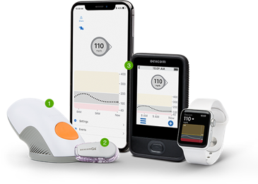
My aim is to predict my glucose levels based on activity data that was collected over a time period of two years using a Fitbit
device and a Dexcom CGM
Three major variables at play:
- Carbohydrate consumption
- Insulin administration
- Levels of physical activity
Of these three variables, the one with the least power to explain the variability in my blood glucose readings is the level of physical activity. From the data that I collected for this experiement, I was able to create an algorithm that mines the data and conducts feature engineering to determine which predictor variables will most accurately make predictions that I can use to predict critical diabetes-related symptoms before they happen. Here are my successes after this project:
- AdaBoost model to predict whether a low blood glucose event would occur in the next hour with 96% accuracy and a ROC Curve with AUC of 99.5
- Random Forest model predicting the average glucose value for the next hour with a MSE of 29.4
- Gathered valuable insights from general descriptive statistical analysis
In the first phase of this project, I regressed the predictor values onto the hourly average glucose reading and my R-squared was approximately 0.08. In other words, only 8% of the variability in the values we are trying to predict were being explained by the indepedent variables. Pretty weak. While this presents a challenging task for us, this is roughly what I was expecting because it agrees with the narrative that this is the least important of those three factors. If physical activity explains 8% of the variability, the other 92% is explained by the food I have eaten and the amount of insulin I have taken - makes sense. How do we increase the predictive power beyong just 8%? If you think about diabetes management, if I were trying to predict my blood glucose in the next hour, the first thing I would ask is “What is my blood glucose right now?”, and that would be a major factor in my prediction. I introduced lagged variables as predictor variables into the process and the performance of my models improved significantly. Effectively, I am adding an indirect measure of carbohydrate consumption and insulin administration by adding lagged variables which subsequently increases the explanatory power of my predictor variables.
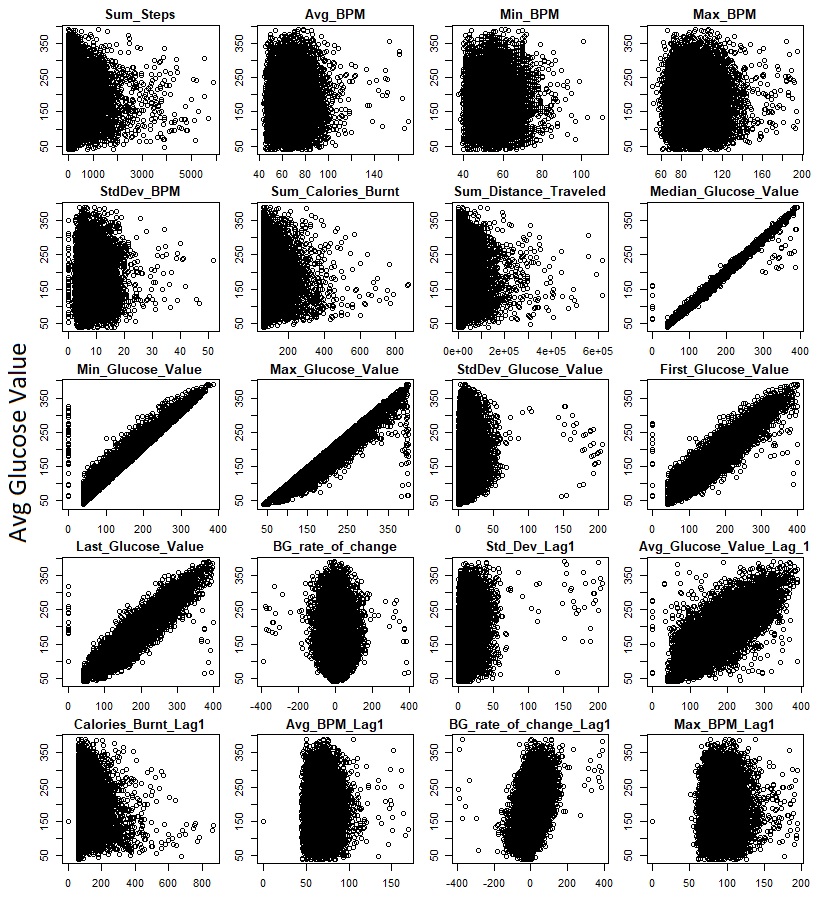
Here’s a look at the relationship between some of the numeric variables I collected and the independent variable that we’re trying to
predict ( y-axis):
Multi Linear Regression
Before I began with some of the more complex analysis, I first wanted to start off simple by running regularizing the variables
through multi-linear regression. Of course, there are some severe limitations to this because I am making the assumption that
the response variable has a linear functional form, but it is a very basic technique and has historically been my first step
when analyzing the explanatory power of independent variables on my response variable. Additionally, the interpretibility of MLR
is very high and will give me a strong indication as to which variables are important during my data exploration phase.
In R, the code looks like this:
#############################################################
################# Multi Linear Reg  #########################
#############################################################
lm.data <-  select(.data = results,c("TimeOfDay","Sum_Steps","Avg_BPM","Min_BPM","Max_BPM","StdDev_BPM","Sum_Calories_Burnt","Sum_Distance_Traveled","Std_Dev_Lag1","Avg_Glucose_Value_Lag_1","Calories_Burnt_Lag1","Avg_BPM_Lag1","LowOccurance_Lag1","HighOccurance_Lag1","BG_rate_of_change_Lag1","Max_BPM_Lag1", "Avg_Glucose_Value"))
set.seed(1)
nobs <- nrow(lm.data) # Determine the number of rows in the dataset.
train <- sample(nobs, 0.7 * nobs)
lm.model <- glm(formula = Avg_Glucose_Value ~ ., data = lm.data[train, ])
###Evaluate by scoring the test set
test <- setdiff(1:nobs, train)  # Collect test data
pr.actuals <- lm.data$Avg_Glucose_Value[test]
preds <- predict(lm.model, newdata = na.omit(lm.data[test, ]))
plot(preds, pr.actuals)
abline(lm(pr.actuals ~ preds), col = "red", lwd = 3)
text(round(coef(lm(pr.actuals ~ preds)),2), x = c(350,375), y = 60)
(lm.std <- sqrt(mean((preds - pr.actuals) ^ 2))) # Calculate RMSE
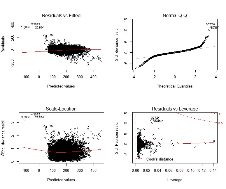
We can see that there are definitely some non-linear components to this data. The calculated RMSE for the test set using MLR is 30.8.
Meaning, we can be confident that 68% of our predictions will fall within a +/- 30.8 window. This is tricky because the units we are
measuring is mg/dL (milligrams of glucose per decilitre) and, as a diabetic, I cannot feel any symptomatic difference between a blood
glucose value of 120 and 150.8, but there is a significant difference between 50 and 80.8.
Here is the graphical performance of Multi Linear Regression:
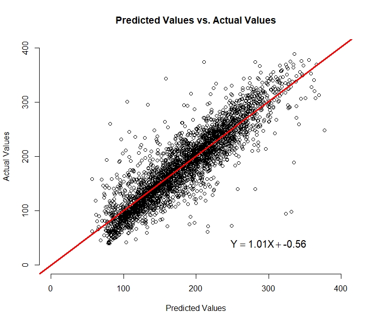
We can see from the graph that the model’s precision begins to deteriorate as we get to the smaller values in the range. Overall, I am
pleased with the performance of this very simple model and the result whereby we have a somewhat linear relationship between the actual
and predicted values with a 45 degree line of best fit. This is what we would hope to see from our model. From the equation displayed
on the chart that was created by regressing the actual values onto the predicted values, we can see that (on average) for every 1 unit
increase of our actual value, there is a one unit increase of our predicted value. The next step is to try some different modeling
techniques to see if we can increase the accuracy of our predictions.
Random Forest
#############################################################
################# Random Forest  ##########################
#############################################################
rf.data <-  select(.data = results, c("TimeOfDay","Sum_Steps","Avg_BPM","Min_BPM","Max_BPM","StdDev_BPM","Sum_Calories_Burnt","Sum_Distance_Traveled","Std_Dev_Lag1","Avg_Glucose_Value_Lag_1","Calories_Burnt_Lag1,"Avg_BPM_Lag1","LowOccurance_Lag1","HighOccurance_Lag1","BG_rate_of_change_Lag1","Max_BPM_Lag1", "Avg_Glucose_Value"))
set.seed(1)
nobs <- nrow(rf.data) # Determine the number of rows in the dataset.
train <- sample(nobs, 0.7 * nobs)
rf <- randomForest(formula = Avg_Glucose_Value ~ ., data = rf.data[train, ], ntree = 500, mtry = 5, importance = TRUE, localImp = TRUE, na.action = na.roughfix, replace = FALSE)
head(rf$predicted, 25)
importance(rf)[order(importance(rf)[, "%IncMSE"], decreasing = T), ]  #Display Variable Importance
###Examine Error Rates for the Trees
head(rf$mse)
plot(rf, col = "red", lwd = 3, main = "Error Rates for Random Forest")  # Plot the error rate against the number of trees.
legend("topright", "OOB Error Rate", lty = 1, col = "red", lwd = 3)
min.err <- min(rf$mse)  # Determine the minimum error rate for Out Of Bag.
min.err.idx <- which(rf$mse == min.err)  # Determine the index corresponding to minimum error rate for Out Of Bag.
min.err.idx
rf$mse[min.err.idx[1]]  # Return the error rates for each of OOB, 0 and 1 corresponding to minimum error rate for Out Of Bag.
###Rebuild the forest with the number of trees that minimizes the OOB error rate - use the first one if there are more than one
rf <- randomForest(formula = Avg_Glucose_Value ~ ., data = rf.data[train,], ntree = min.err.idx[1], mtry = 5, importance = TRUE, localImp = TRUE, na.action = na.roughfix, replace = FALSE)
plot(rf, col = "red", lwd = 3, main = "Error Rates for Random Forest")  # Plot the error rate against the number of trees.
legend("topright", "OOB Error Rate", lty = 1, col = "red", lwd = 3)
###Evaluate by scoring the test set
test <- setdiff(1:nobs, train)  # Collect test data
pr.actuals <- rf.data$Avg_Glucose_Value[test]
preds <- predict(rf, newdata = na.omit(rf.data[test, ]))
plot(preds, pr.actuals)
abline(lm(pr.actuals ~ preds), col = "red", lwd = 3)
coef(lm(pr.actuals ~ preds))
(rf.std <- sqrt(mean((preds - pr.actuals) ^ 2))) # Calculate RMSE
AdaBoost
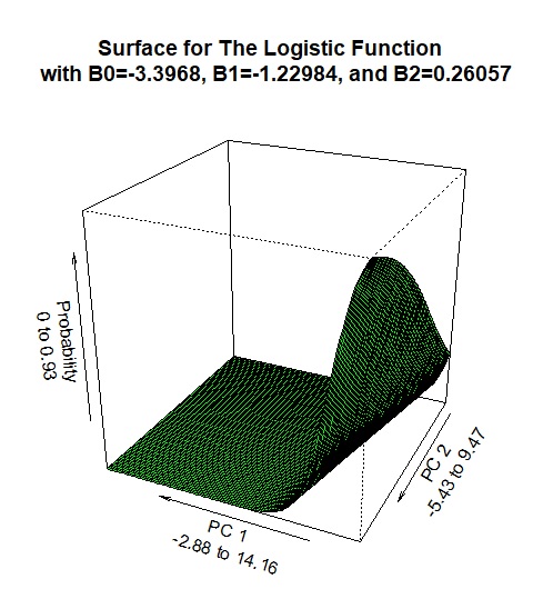
Now we are going to attempt a classfication problem. In other words, we are going to try and predict whether there is (or is not) the occurrence of a low blood glucose reading within a given value. Using Adaptive Boosting is similar to a logistic regression problem where we are looking for the maximum liklihood and our target response is a value between 0 and 1, which replicates a probability. The following graphic is a logistic function, but a similar process is used to determine a predicted class. The axes in this visualization of two of the significant principal components (which is interpretted as a linear combination of multiple variables). In the case of Logistic Regression, as each of the numeric values of the two variables increases or decreases, the response variable (which in this case is a probability between 0 and 1) and moves along this 3-dimensional logistic function. The probability is measured on the vertical axis in this graphic.
#############################################################
##################### AdaBoost ##############################
#############################################################
# Predicting if there is at least one blood sugar in a given hour
# which is indicated by the binary variable LowOccurance which is number 31
ada.data <-  select(.data = results c("TimeOfDay","Sum_Steps","Avg_BPM","Min_BPM","Max_BPM","StdDev_BPM","Sum_Calories_Burnt","Sum_Distance_Traveled","Std_Dev_Lag1","Avg_Glucose_Value_Lag_1","Calories_Burnt_Lag1","Avg_BPM_Lag1","LowOccurance_Lag1","HighOccurance_Lag1","BG_rate_of_change_Lag1","Max_BPM_Lag1","LowOccurance"))
nobs <- nrow(ada.data)
train <- sample(nobs, 0.7*nobs)
bm<- ada(formula=LowOccurance ~ .,data=ada.data[train,], iter=50, bag.frac=0.5, control=rpart.control(maxdepth=30,cp=0.01, minsplit=20,xval=10))
print(bm)
# Evaluate by scoring the training set
prtrain <- predict(bm, newdata=ada.data[train,])
prtrainProbs <- predict(bm, newdata=ada.data[train,], type = "prob")
table(ada.data[train,"LowOccurance"], prtrain,dnn=c("Actual", "Predicted"))
round(100* table(ada.data[train,"LowOccurance"], prtrain,dnn=c("% Actual", "% Predicted"))/length(prtrain),1)
#ROC Curve
aucc <- roc.area(as.integer(as.factor(ada.data[train, "LowOccurance"]))-1,prtrainProbs[,2])
aucc$A
aucc$p.value                #null hypothesis: aucc=0.5
roc.plot(as.integer(as.factor(ada.data[train,"LowOccurance"]))-1,prtrainProbs[,2], main="ROC Plot for Adaptive Boosting Classifier")
# Evaluate by scoring the test set
prtest <- predict(bm, newdata=ada.data[-train,])
table(ada.data[-train,"LowOccurance"], prtest,dnn=c("Actual", "Predicted"))
round(100* table(ada.data[-train,"LowOccurance"], prtest,dnn=c("% Actual", "% Predicted"))/length(prtest),1)
#ada.data[1:100,]
probs <- predict(bm, newdata = ada.data[-train,], "prob")
prtest2 <- rep(0, nrow(ada.data[-train,]))
prtest2[which(predict(bm, newdata = ada.data[-train,], "prob")[,2] > 0.3)] <- 1
round(100* table(ada.data[-train,"LowOccurance"], prtest2,dnn=c("% Actual", "% Predicted"))/length(prtest),1)